W3cubDocs
/NumPy 1.13numpy.histogram2d
-
numpy.histogram2d(x, y, bins=10, range=None, normed=False, weights=None)[source] -
Compute the bi-dimensional histogram of two data samples.
Parameters: x : array_like, shape (N,)
An array containing the x coordinates of the points to be histogrammed.
y : array_like, shape (N,)
An array containing the y coordinates of the points to be histogrammed.
bins : int or array_like or [int, int] or [array, array], optional
The bin specification:
- If int, the number of bins for the two dimensions (nx=ny=bins).
- If array_like, the bin edges for the two dimensions (x_edges=y_edges=bins).
- If [int, int], the number of bins in each dimension (nx, ny = bins).
- If [array, array], the bin edges in each dimension (x_edges, y_edges = bins).
- A combination [int, array] or [array, int], where int is the number of bins and array is the bin edges.
range : array_like, shape(2,2), optional
The leftmost and rightmost edges of the bins along each dimension (if not specified explicitly in the
binsparameters):[[xmin, xmax], [ymin, ymax]]. All values outside of this range will be considered outliers and not tallied in the histogram.normed : bool, optional
If False, returns the number of samples in each bin. If True, returns the bin density
bin_count / sample_count / bin_area.weights : array_like, shape(N,), optional
An array of values
w_iweighing each sample(x_i, y_i). Weights are normalized to 1 ifnormedis True. Ifnormedis False, the values of the returned histogram are equal to the sum of the weights belonging to the samples falling into each bin.Returns: H : ndarray, shape(nx, ny)
The bi-dimensional histogram of samples
xandy. Values inxare histogrammed along the first dimension and values inyare histogrammed along the second dimension.xedges : ndarray, shape(nx+1,)
The bin edges along the first dimension.
yedges : ndarray, shape(ny+1,)
The bin edges along the second dimension.
See also
-
histogram - 1D histogram
-
histogramdd - Multidimensional histogram
Notes
When
normedis True, then the returned histogram is the sample density, defined such that the sum over bins of the productbin_value * bin_areais 1.Please note that the histogram does not follow the Cartesian convention where
xvalues are on the abscissa andyvalues on the ordinate axis. Rather,xis histogrammed along the first dimension of the array (vertical), andyalong the second dimension of the array (horizontal). This ensures compatibility withhistogramdd.Examples
>>> import matplotlib as mpl
>>> import matplotlib.pyplot as plt
Construct a 2-D histogram with variable bin width. First define the bin edges:
>>> xedges = [0, 1, 3, 5]
>>> yedges = [0, 2, 3, 4, 6]
Next we create a histogram H with random bin content:
>>> x = np.random.normal(2, 1, 100)
>>> y = np.random.normal(1, 1, 100)
>>> H, xedges, yedges = np.histogram2d(x, y, bins=(xedges, yedges))
>>> H = H.T  # Let each row list bins with common y range.
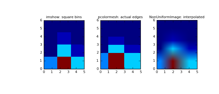
imshowcan only display square bins:>>> fig = plt.figure(figsize=(7, 3)) >>> ax = fig.add_subplot(131, title='imshow: square bins') >>> plt.imshow(H, interpolation='nearest', origin='low', ... extent=[xedges[0], xedges[-1], yedges[0], yedges[-1]])
pcolormeshcan display actual edges:>>> ax = fig.add_subplot(132, title='pcolormesh: actual edges', ... aspect='equal') >>> X, Y = np.meshgrid(xedges, yedges) >>> ax.pcolormesh(X, Y, H)
NonUniformImagecan be used to display actual bin edges with interpolation:>>> ax = fig.add_subplot(133, title='NonUniformImage: interpolated', ... aspect='equal', xlim=xedges[[0, -1]], ylim=yedges[[0, -1]]) >>> im = mpl.image.NonUniformImage(ax, interpolation='bilinear') >>> xcenters = (xedges[:-1] + xedges[1:]) / 2 >>> ycenters = (yedges[:-1] + yedges[1:]) / 2 >>> im.set_data(xcenters, ycenters, H) >>> ax.images.append(im) >>> plt.show()
(Source code, png, pdf)
© 2008–2017 NumPy Developers
Licensed under the NumPy License.
https://docs.scipy.org/doc/numpy-1.13.0/reference/generated/numpy.histogram2d.html